MPC with a Differentiable Forward Model: An Implementation with Jax
Published:
Intro
In a recent project for MECS6616 Robot Learning, I got hands-on experience for Model Predictive Control (MPC). To solve the problem, the use of constant action and pseudo-gradient is a recommended method, and it truly provides simple yet good enough solutions. However, the project instructions also hinted at another prospect: a differentiable forward model could help, since you can always compute numerical gradients. This piqued my curiosity - could we directly compute the gradient with respect to action given the evaluation metric? And if so, how could we implement this practically?
With these questions in mind, I embarked on a journey to explore the use of differentiable programming in the context of MPC. My tool of choice was Jax, a high-performance machine learning library. The journey in the end, however, reveals that direct calculation of numerical gradients from the target metric doesn’t necessarily equate to better performance. This realization reminded me of a 2017 paper by OpenAI on evolution strategies, which I would like to share in the future.
In this blog&tutorial, I’ll share my implementation and provide a step-by-step guide to implementing MPC with a differentiable forward model using Jax.
Background
MPC
Model Predictive Control (MPC) is a control strategy that involves the use of an optimization algorithm to determine the optimal control inputs to a system. The optimization problem is formulated based on a model of the system, a cost function, and constraints on the system states and inputs. The control inputs from the optimal solution are then applied to the system, and the process is repeated at the next time step. This strategy allows MPC to anticipate future events and act accordingly.
Forward model
The forward model, which is a function that takes the current state of the system and the action given to the robot as input, and outputs the next state of the system.
\[x_{k+1}=f(x_k,u_k)\]Where \(x_k\) is the state of the system at time step $k$, \(u_k\) is the action / command given to the robot at time step $k$.
Cost function and Goal
Cost functions can be user-defined, for instance, the cost function \(j(x,u)\) is the cost of a state and action, \(j_F(x)\) is the cost of the terminal state. The goal is the optimization objective, and the target is to find an action sequence that minimize the objective. A goal $j$ could be: \(J=\sum_{i=k}^{N-1}j(x_i,u_i)+j_F(x_N)\), where $N$ is the control horizon.
JAX
JAX is a Python library developed by Google that provides capabilities for efficient and easily differentiable numerical computation. JAX extends the familiar NumPy interface with automatic differentiation, enabling users to compute gradients with minimal changes to their code. It also includes support for just-in-time compilation via XLA, making it possible to develop efficient, speed-optimized code in Python.
I think the coolest feature of JAX is the grad, which differentiate a function. Here is a simple example:
from jax import numpy as jnp
from jax import grad

def tanh(x):
  return jnp.tanh(x)

grad_tanh = grad(tanh)
print(grad_tanh(2.0))
# 0.070650816
grad takes a function and returns a function. If you have a Python function f that evaluates the mathematical function , then grad(f) is a Python function that evaluates the mathematical function \(\nabla f\). That means grad(f)(x) represents the value \(\nabla f(x)\).
And since grad operates on functions, you can apply it to its own output to differentiate as many times as you like:
print(grad(grad(jnp.tanh))(2.0))
print(grad(grad(grad(jnp.tanh)))(2.0))
# -0.13621868
# 0.25265405
Implementation
Problem formulation
Given an n linked robot arm and the ground truth forward dynamics, the target is to design a controller that could minimizes the distance of end effector to the goal position and the velocity of the end effector at the terminal state.
In a colab notebook:
!git clone https://github.com/roamlab/mecs6616_sp23_project4.git
!mv /content/mecs6616_sp23_project4/* /content/
!pip install ray
The differentiable forward model is implemented as below:
import jax
from jax import numpy as jnp
from arm_dynamics_teacher import ArmDynamicsTeacher
from geometry import rot, xaxis, yaxis


class DifferentiableArmDynamicsTeacher(ArmDynamicsTeacher):
    def dynamics_step(self, state, action, dt):
        """ Forward simulation using Euler method """
        left_hand, right_hand = self.constraint_matrices(state, action)
        a, qdd = self.solve(left_hand, right_hand)
        new_state = self.integrate_euler(state, a, qdd, dt)
        return new_state

    def constraint_matrices(self, state, action):
        """ Contructs the constraint matrices from state """
        # Computes variables dependent on state required to construct constraint matrices
        num_vars = self.num_var()
        q = self.get_q(state)
        theta = self.compute_theta(q)
        qd = self.get_qd(state)
        omega = self.compute_omega(qd)
        vel_0 = self.get_vel_0(state)
        vel = self.compute_vel(vel_0, omega, theta)
        vel_com = self.compute_vel_com(vel, omega)

        left_hand = None
        right_hand = None

        # Force equilibrium constraints
        for i in range(0, self.num_links):
            cl = np.zeros((2, num_vars))
            cl[0:2, self.idx_f(i):self.idx_f(i + 1)] = -1 * np.eye(2)
            cl[0:2, self.idx_a(i):self.idx_a(i + 1)] = -1 * self.link_masses[i] * np.eye(2)
            cl[1, self.idx_omdot(i)] = -1 * 0.5 * self.link_lengths[i] * self.link_masses[i]
            if i < self.num_links - 1:
                cl[0:2, self.idx_f(i + 1):self.idx_f(i + 2)] = rot(q[i + 1])
            cr = np.zeros((2, 1))
            # gravity
            if self.gravity:
                cr = cr + (-1 * 9.8 * self.link_masses[i]) * (np.dot(rot(-1 * theta[i]), (-1 * yaxis())))
            # centrifugal force
            cr[0] = cr[0] + (-1) * (omega[i] * omega[i] * 0.5 * self.link_lengths[i] * self.link_masses[i])
            if i == 0:
                left_hand = cl
                right_hand = cr
            else:
                left_hand = np.concatenate((left_hand, cl))
                right_hand = np.concatenate((right_hand, cr))

        # Torque equilibrium constraints
        for i in range(0, self.num_links):
            cl = np.zeros((1, num_vars))
            # the y component of the force
            cl[0, self.idx_f(i) + 1] = self.link_lengths[i] * 0.5
            # inertial torque
            cl[0, self.idx_omdot(i)] = -1 * self.link_inertias[i]
            if i < self.num_links - 1:
                # the y component
                cl[0, self.idx_f(i + 1):self.idx_f(i + 2)] = self.link_lengths[i] * 0.5 * rot(q[i + 1])[1, :]
            left_hand = np.concatenate((left_hand, cl))
            cr = np.zeros((1, 1))
            right_hand = np.concatenate((right_hand, cr))
            # viscous friction depends on the mode, implemented in ArmDynamics & SnakeDynamics

        # Linear acceleration constraints
        for i in range(1, self.num_links):
            cl = np.zeros((2, num_vars))
            cl[0:2, self.idx_a(i):self.idx_a(i + 1)] = -1 * np.eye(2)
            cl[0:2, self.idx_a(i - 1):self.idx_a(i)] = rot(-1 * q[i])
            cl[0:2, self.idx_omdot(i - 1):self.idx_omdot(i)] = self.link_lengths[i - 1] * (
                np.dot(rot(-1 * q[i]), (1 * yaxis())))
            left_hand = np.concatenate((left_hand, cl))
            cr = -1 * self.link_lengths[i - 1] * omega[i - 1] * omega[i - 1] * (np.dot(rot(-1 * q[i]), (-1 * xaxis())))
            right_hand = np.concatenate((right_hand, cr))

        assert left_hand.shape == (self.num_var() - 2, self.num_var())
        assert right_hand.shape == (self.num_var() - 2, 1)

        # Joint viscous friction
        for i in range(self.num_links):
            right_hand[self.idx_tau_eqbm(i)] += qd[i] * self.joint_viscous_friction

        # Linear acceleration of joint-0 must be zero
        cl = np.zeros((2, self.num_var()))
        cl[0:2, self.idx_a(0):self.idx_a(1)] = np.eye(2)
        left_hand = np.concatenate((left_hand, cl))
        cr = np.zeros((2, 1))
        right_hand = np.concatenate((right_hand, cr))

        assert left_hand.shape == (5 * self.num_links, 5 * self.num_links)
        assert right_hand.shape == (5 * self.num_links, 1)

        # Apply torques
        right_hand = jnp.array(right_hand)
        tau = action
        tau_shift = jnp.roll(action, shift=-1)
        tau_shift.at[-1].set(0.)
        tau_diff = tau_shift - tau
        for i in range(self.num_links):
            right_hand = right_hand.at[self.idx_tau_eqbm(i), 0].add(tau_diff[i, 0])

        return left_hand, right_hand

    def solve(self, left_hand, right_hand):
        """ Solves the constraint matrices to compute accelerations """
        x = jnp.linalg.solve(left_hand, right_hand)
        self.residue = jnp.linalg.norm(jnp.dot(left_hand, x) - right_hand) / self.num_var()
        residue = jnp.linalg.norm(jnp.dot(left_hand, x) - right_hand) / self.num_var()
        if residue > self.residue_limit:
            print('cannot solve, residue {} exceeds limit {}'.format(residue, self.residue_limit))
            self.residue_limit_flag = True
        a = x[self.idx_a(0):self.idx_a(self.num_links)]
        omdot = x[self.idx_omdot(0):self.idx_omdot(self.num_links)]
        qdd = omdot.copy()
        for i in range(self.num_links - 1, 0, -1):
            qdd = qdd.at[i].add(-qdd[i - 1])
        return a, qdd

    def integrate_euler(self, state, a, qdd, dt):
        """ Integrates using Euler method """
        # Compute state dependent variables needed for integration
        q = self.get_q(state)
        qd = self.get_qd(state)

        qd_new = qd + qdd * dt
        q_new = q + 0.5 * (qd + qd_new) * dt

        new_state = jnp.vstack([q_new, qd_new])
        return new_state

    def compute_theta(self, q):
        return jnp.cumsum(q, axis=0)

    def compute_pos(self, pos_0, theta):
        pos = []
        pos.append(pos_0)
        for i in range(1, self.num_links):
            pos.append(pos[i - 1] + jnp.dot(self.rot(theta[i - 1]), self.link_lengths[i - 1] * xaxis()))
        pos = jnp.vstack(pos)
        return pos

    def compute_fk(self, state):
        pos_0 = self.get_pos_0(state)
        q = self.get_q(state)
        theta = self.compute_theta(q)
        pos = self.compute_pos(pos_0, theta)
        pos_ee = jnp.array([pos[2*(self.num_links-1)], pos[2*(self.num_links-1)+1]])
        pos_ee = pos_ee + jnp.dot(self.rot(theta[self.num_links - 1]), self.link_lengths[self.num_links - 1] * xaxis())
        return pos_ee

    def compute_vel(self, vel_0, omega, theta):
        vel = []
        vel.append(vel_0)
        vel_world = []
        vel_world.append(jnp.dot(self.rot(theta[0]), vel_0))
        for i in range(1, self.num_links):
            vel_world.append(vel_world[i - 1] + (jnp.dot(self.rot(theta[i - 1]), omega[i - 1] * self.link_lengths[i - 1] * yaxis())))
            vel.append(jnp.dot(self.rot(-1.0 * theta[i]), vel_world[i]))
        vel = jnp.vstack(vel)
        return vel

    def rot(self, theta):
        R = jnp.array([[jnp.cos(theta), -jnp.sin(theta)],
                       [jnp.sin(theta), jnp.cos(theta)]]).reshape(2, 2)
        return R
Based on the differentiable forward model, the MPC is implemented as:
from collections import defaultdict
import numpy as np
import random
seed = 0
random.seed(seed)
np.random.seed(seed)

def calc_dist(action, dynamics, state, goal, dt):
    next_state = dynamics.dynamics_step(state, action, dt)
    pos_ee = dynamics.compute_fk(next_state)
    dist = jnp.linalg.norm(goal - pos_ee)
    # vel_ee = jnp.linalg.norm(arm.dynamics.compute_vel_ee(next_state))
    return dist

class MPC:

  def __init__(self,
               time_limit: float = 5.,
               dt: float = 0.01,
               scale: float = 1.,
               num_controls: int = None):
    self.dt = dt
    self.control_horizon = 10
    # Define other parameters here
    self.num_steps = round(time_limit/dt)
    self.num_controls = len([i for i in range(self.num_steps) if i % self.control_horizon == 0]) if not num_controls else num_controls
    self.scale = scale

  def compute_action(self, dynamics, state, goal, action):
    # Put your code here. You must return an array of shape (num_links, 1)

    # Don't forget to comment out the line below
    # raise NotImplementedError("MPC not implemented")
    best_action = self._planning(dynamics, action, state, goal)
    return best_action

  def _planning(self, dynamics, action, initial_state, goal):
    state = initial_state
    gradient = 0.
    for i in range(self.num_controls):
      state = dynamics.dynamics_step(state, action, self.dt)
      gradient += jax.grad(calc_dist, argnums=0)(action, dynamics, state, goal, self.dt)
    print(f'grad: {gradient},')
    print(f'action: {action}')
    best_action = action - np.array(gradient) * self.scale
    return best_action
To test the MPC controller, you can use this part of code:
import sys
import numpy as np
from arm_dynamics_teacher import ArmDynamicsTeacher
from robot import Robot
from render import Renderer
from score import *
import torch
import time
import math
np.set_printoptions(suppress=True)
# Teacher arm with 3 links
dynamics_teacher = DifferentiableArmDynamicsTeacher(
num_links=3,
link_mass=0.1,
link_length=1,
joint_viscous_friction=0.1,
dt=0.01)
arm = Robot(dynamics_teacher)
arm.reset()
gui = False
if gui:
renderer = Renderer()
time.sleep(1)
# Controller
controller = MPC(time_limit=5, num_controls=10, scale=1.)
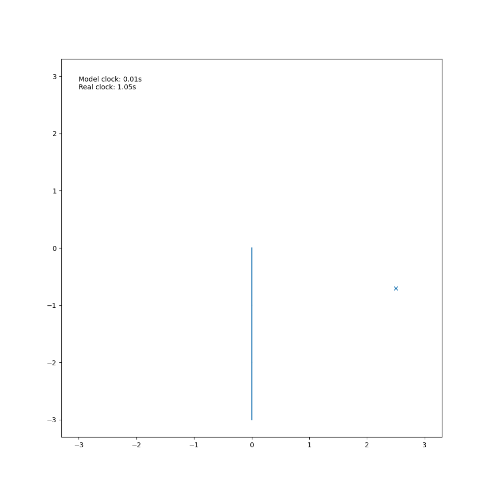
# Resetting the arm will set its state so that it is in the vertical position,
# and set the action to be zeros
arm.reset()
# Choose the goal position you would like to see the performance of your controller
goal = np.zeros((2, 1))
goal[0, 0] = 2.5
goal[1, 0] = -0.7
arm.goal = goal
dt = 0.01
time_limit = 5
num_steps = round(time_limit/dt)
# Control loop
action = np.zeros((3,1))
for s in range(num_steps):
t = time.time()
arm.advance()
if gui:
renderer.plot([(arm, "tab:blue")])
time.sleep(max(0, dt - (time.time() - t)))
if s % controller.control_horizon==0:
state = arm.get_state()
# Measuring distance and velocity of end effector
pos_ee = dynamics_teacher.compute_fk(state)
dist = np.linalg.norm(goal-pos_ee)
vel_ee = np.linalg.norm(arm.dynamics.compute_vel_ee(state))
print(f'At timestep {s}: Distance to goal: {dist}, Velocity of end effector: {vel_ee}')
action = controller.compute_action(arm.dynamics, state, goal, action)
# print(f'Action: {action}')
arm.set_action(action)