What are the Effective Deep Learning Models for Tabular Data?

27 minute read

Published: March 13, 2022

This week, I would like to share a paper published at NeurIPS 2021. When dealing with tabular data, I often find myself perplexed. On one hand, I am unsure which deep learning frameworks are better suited for this task, and on the other hand, I am uncertain whether the time-consuming process of training a model can outperform the easily accessible GBDT family of models such as XGBoost and LightGBM. However, this paper provides a detailed and comprehensive comparison of deep learning algorithms and GBDT models on tabular data. It introduces new baselines and presents a novel architecture that outperforms other deep learning models. I have gained a lot from this paper and would like to share it with you.

Original Paper Information
Title: Revisiting Deep Learning Models for Tabular Data
Author: Yury Gorishniy, Ivan Rubachev, Valentin Khrulkov, Artem Babenko
Code: https://github.com/yandex-research/rtdl

Background

Deep learning has achieved significant success in the domains of image, audio, and text data, which has sparked interest in applying deep learning to tabular data. Tabular data refers to data points represented as vectors with diverse features, stored in a tabular form. Such data is commonly encountered in industrial applications and machine learning competitions.

However, despite the proliferation of deep learning models applied to tabular data, previous studies lacked sufficient benchmarks and suffered from issues such as insufficient comparisons and inconsistent datasets. Additionally, while there have been novel architectures proposed in this field, there is still a lack of a simple, reliable, and competitive baseline. MLP remains the main baseline in this field, but it falls short in terms of competitiveness, despite its simplicity.

Therefore, the authors compared mainstream deep learning models on various commonly used datasets with the same training framework. The authors also proposed two simple yet competitive frameworks: ResNet-like MLP, which is easy to tune but is outperformed by other models across multiple datasets, and FT-Transformer, which is a simple modification of the Transformer architecture and exhibits superior performance on the majority of datasets. Finally, the paper compared several state-of-the-art deep learning models with GBDT, concluding that neither approach is globally superior, and both have their strengths and weaknesses.

Models to compare

$\newcommand{\mlp}{\mathrm{MLP}} \newcommand{\mlpb}{\mathrm{MLPBlock}} \newcommand{\lin}{\mathrm{Linear}} \newcommand{\drop}{\mathrm{Dropout}} \newcommand{\relu}{\mathrm{ReLU}} \newcommand{\resn}{\mathrm{ResNet}} \newcommand{\resb}{\mathrm{ResNetBlock}} \newcommand{\pred}{\mathrm{Prediction}} \newcommand{\bn}{\mathrm{BatchNorm}} \newcommand{\stack}{\mathrm{stack}} \newcommand{\fttrans}{\mathrm{FT-Transformer}} \newcommand{\fttb}{\mathrm{Block}} \newcommand{\ft}{\mathrm{FeatureTokenizer}} \newcommand{\ffn}{\mathrm{FFN}} \newcommand{\rpn}{\mathrm{ResidualPreNorm}} \newcommand{\norm}{\mathrm{Norm}} \newcommand{\act}{\mathrm{Activation}} \newcommand{\module}{\mathrm{Module}} \newcommand{\mhsa}{\mathrm{MHSA}} \newcommand{\acls}{\mathrm{AppendCLS}} \newcommand{\layern}{\mathrm{LayerNorm}}$ This section describes the models used for comparison. There are some symbols and concepts that need to be clarified:

The paper focuses on supervised learning problems. $D={(x_i,y_i)}$ represents the dataset, where $x_i=(x_i^{num},x_i^{cat})$ represents the numerical and categorical features respectively, and $yi$ represents the corresponding labels. There are a total of $k$ features. The dataset is divided into three disjoint subsets: $D=D_{train} \cup D_{val} \cup D_{test}$. $D_{train}$ is used for model training, $D_{val}$ is used for hyperparameter tuning and early stopping, and $D_{test}$ is used for final evaluation.

The tasks encompass three types: binary classification, regression, and multi-class classification.

1. MLP

Each Multilayer Perceptron (MLP) block consists of three parts:

One linear layer;
ReLU activation;
Dropout layer.

Multiple MLP blocks are nested together, and the output is passed through a final linear layer. $\mlp(x)=\lin(\mlpb(...(\mlpb(x))))$

2. ResNet-like MLP

The paper introduces a simple variant of ResNet, and the structure of the ResNet model in the paper is as follows: $\begin{align} \resn(x) & =\pred(\resb(...(\resb(\lin(x))))) \\ \resb(x) & =x+\drop(\lin(\drop(\relu(\lin(\bn(x)))))) \\ \pred(x) & =\lin(\relu(\bn(x))) \end{align}$ It consists of multiple nested residual blocks, followed by batch normalization, ReLU activation, and a linear layer for output. Each residual block includes batch normalization, a linear layer, ReLU activation, Dropout, another linear layer, Dropout, and a residual connection.

3. FT-Transformer

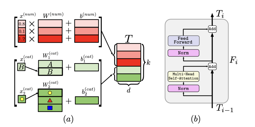
The authors proposed the FT-Transformer (Feature Tokenizer Transformer) architecture, as shown below. It consists of two parts: the first part involves mapping all the features to embedding vectors, while the second part applies a series of Transformer blocks to these vectors.

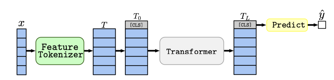
The Feature Tokenizer block performs a linear transformation and adds bias on numerical features, with independent weights for each numerical feature. For categorical variables, each category is mapped to a distinct vector, and the categorical variables are treated independently. This process results in a $k\times d$-dimensional vector $T$. The formula can be expressed as follows: $\begin{align} & T_j^{(num)} = b_j^{(num)}+x_j \cdot W_j^{(num)} & \in \mathbb{R}^d,\\ & T_j^{(cat)} = b_j^{(cat)}+e_j^TW_j^{(cat)} & \in\mathbb{R}^d, \\ & T = \stack[T_1^{(num)},...,T_{k^{(num)}}^{(num)},T_1^{(cat)},...,T_{k^{(cat)}}^{(cat)}] & \in \mathbb{R}^{k\times d}. \end{align}$

The Transformer block starts by adding a [CLS] token to the beginning of the vector $T$. Each block in the Transformer consists of a multi-head self-attention and a feed-forward network. Both parts of the block undergo layer normalization and residual connections. $\begin{align} \fttrans(x)&=\pred(\fttb(...(\fttb(\acls(\ft(x)))))) \\ \fttb(x)&=\rpn(\ffn,\rpn(\mhsa,x)) \\ \rpn(\module, x) &= x + \drop(\module(\norm(x))) \\ \ffn(x) &= \lin(\drop(\act(\lin(x)))) \end{align}$ The final prediction is made using the extracted [CLS] vector after passing through multiple layers, which are layer normalization, ReLU activation, and a linear layer. $\hat{y}=\lin(\relu(\layern(T_L^{[CLS]}))).$

4. Other models

In this section, the authors briefly mention several models: SNN, NODE, TabNet, GrowNet, DCN V2, AutoInt, XGBoost, and CatBoost.

It is mentioned in the appendix that NODE, TabNet, and GrowNet utilize official open-source implementations. As for the other deep learning models, they were implemented by the authors themselves, and the source code can be found in their open-source repository.

Experiments

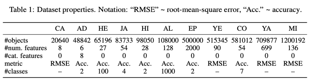
1. Datasets

Apart from Appendix, 11 publicly available datasets are compared in the paper. Each dataset undergoes a single data split, and all models are trained, validated, and tested on the exact same data to ensure fair comparison.

2. Implementation details

Preprocessing:
- Data preprocessing has a significant impact on the performance of deep learning models. By default, the quantile transform from scikit-learn is used. Normalization is applied to the Helena and ALOI datasets, while for the Epsilon dataset, it was found that preprocessing had a detrimental effect, so the original data was used. The regression targets are standardized.
Hyperparameter Tuning:
- Hyperparameters are tuned using a validation set. The authors mention the use of the Optuna tool for Bayesian optimization, which has been shown to outperform random search (Turner et al., 2021). The comparisons in the main body of the paper are limited to a specific number of iterations, and comparisons with limited time are provided in the appendix.
Evaluation:
- The experiments are run with different random seeds, and the performance on the test set is averaged over 15 runs.
Ensemble Methods:
- Ensemble methods are considered in the experiments. For each model, the 15 individual models are divided into three disjoint groups, and the outputs of the models within each group are averaged.
Neural Networks:
- For classification problems, cross-entropy loss is used, while for regression problems, mean squared error is used. TabNet and GrowNet follow the original papers and use the Adam optimizer, while the others use AdamW. All models terminate training if there is no improvement on the validation set for 17 consecutive epochs.
Handling Categorical Variables:
- For XGBoost, one-hot encoding is used, while CatBoost utilizes its built-in methods for categorical variable handling. For neural networks, embeddings of the same dimensions are used, following the approach described in the FT-Transformer.

3. Result

3.1 Deep learning models comparison

The result is shown below:

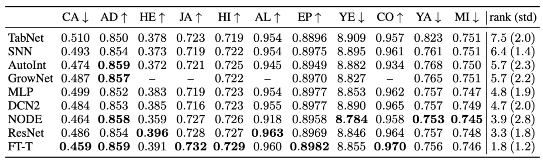
To summarize,

MLP remains a good sanity check.
ResNet serves as an effective baseline, as no other model consistently outperforms it.
Fine-tuning can make MLP and ResNet competitive, so the authors recommend tuning the parameters of the baselines when feasible. They also mention the helpfulness of Optuna in parameter tuning.
Next, the authors found that the NODE model performs well on multiple tasks. However, it has a larger parameter count compared to ResNet and FT-Transformer, and it employs a framework similar to ensemble learning. Therefore, the authors further compared the performance of NODE, ResNet, and FT-Transformer using ensembling.

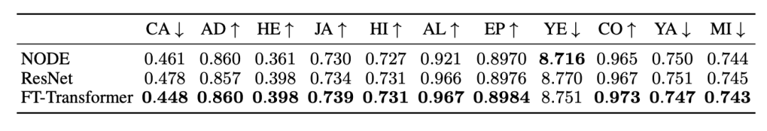
Figure 5. Ensemble deep learning models comparison. Bold indicates the best-performing model for each task.

It can be observed that ResNet and FT-Transformer benefit more from ensembling, while NODE’s improvement is relatively smaller. Additionally, FT-Transformer consistently outperforms the NODE model.

3.2 Deep learning vs GBDT

In this section, all deep learning models are compared with GBDT models in ensemble ways. The results are as follows:

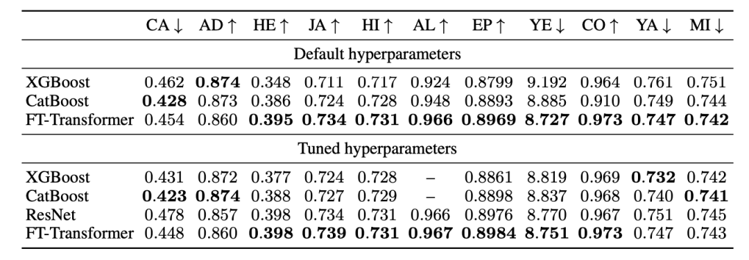
Ensemble deep learning models vs GBDT — Figure 6. Ensemble deep learning models and GBDT models comparison. Bold indicates the best-performing model for each task.

The authors compared the performance of default and tuned parameters. The performance of default parameters is important since it is a common scenario in practice. It can be seen that the ensemble of FT-Transformer with default parameters performs on par with the tuned FT-Transformer.

After tuning the parameters, GBDT dominates in some datasets, and the difference in performance is significant. This indicates that there is no general superiority between deep learning and GBDT. However, for multi-class classification problems with a larger number of classes, GBDT is not particularly suitable. For example, in the case of Helena with 100 classes, GBDT’s performance after tuning is unsatisfactory, and for ALOI with 1000 classes, the training process is slow and it becomes challenging to tune the GBDT model.

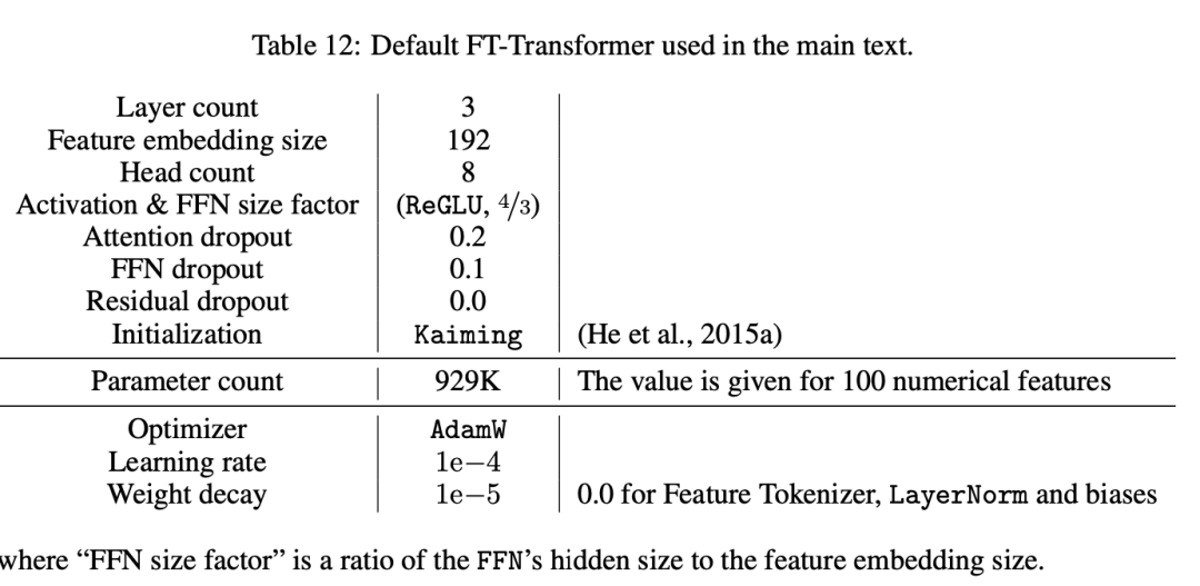
The default parameters of FT-Transformer is given in the Appendix:

4. Inspiring question: When is FT-Transformer better than ResNet?

The author observed that on datasets where GBDT outperforms ResNet, FT-Transformer also exhibits a larger advantage over ResNet. On other datasets, the performance of the two models is relatively close, which the author observed in both single-model and ensemble settings.

Therefore, the author conducted a series of synthetic tasks to demonstrate when FT-Transformer is better than ResNet, ranging from negligible performance difference to significant gaps.

First, the author generated and fixed a series of data points ${x_i}$ and performed a single train-validate-test split. Two regression targets were defined: $f_{GBDT}$, which is expected to be simpler for GBDT, and $f_{DL}$, which is expected to be simpler for ResNet. The definitions are as follows:

\[x\sim \mathcal{N}(0,I_k), \\ y=\alpha f_{GBDT}(x)+(1-\alpha)f_{DL}(x).\]

where $f_{GBDT}(x)$ is the average output of 30 randomly generated decision trees, $f_{DL}(x)$ is an MLP with 3 randomly initialized layers. The target $y$ is normalized before training.

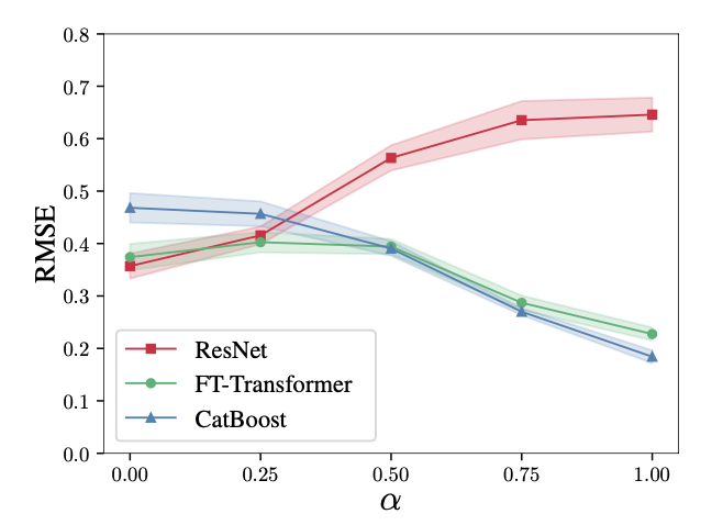
FT-Transformer vs ResNet — Figure 8. 5 experiment results on test set, each alpha represents a task.

It can be observed that on tasks that are simpler for ResNet (small $\alpha$), both deep learning models outperform CatBoost. However, as the tasks become more GBDT-friendly (large $\alpha$), the performance of the ResNet model significantly declines. On the other hand, FT-Transformer exhibits competitive performance across all tasks.

This experiment demonstrates that FT-Transformer is better than ResNet at fitting functions that are based on decision trees. This finding may be related to the previous observations.

5. Ablation Experiments

In this section, the author conducted several ablation experiments on the implementation choices of FT-Transformer.

First, the author compared the AutoInt model, which also maps features to embedding vectors and utilizes self-attention. However, there are differences in the implementation details. AutoInt does not include biases during feature mapping, and its core structure differs significantly from the architecture described in Vaswani et al., 2017, the canonical Transformer. Additionally, AutoInt does not utilize techniques such as adding [CLS] during inference.

Using the same procedure as before, the author examined the performance without adding biases, as shown in the figure:

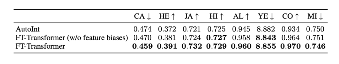
Ablation Transformer — Figure 9. 2 attention mechanism and w/o feature biases comparison.

It can be observed that the core of Transformer is better than AutoInt, and including feature biases yields better results compared to excluding them.

Conclusion

This paper provides a comprehensive comparison of mainstream deep learning models on multiple tabular datasets and improves the baseline standards for deep learning on tabular data. Firstly, it demonstrates the effectiveness of ResNet-like architectures as strong baselines. Secondly, it introduces FT-Transformer, which outperforms other deep learning models on the majority of datasets. Thirdly, through the comparison of deep learning models with GBDT, it reveals that GBDT still dominates on certain datasets.

Appendix

In the appendix, there is still a wealth of noteworthy information. It includes the parameter spaces for hyperparameter tuning of each model, which is not elaborated here. Instead, I will highlight some additional experiments.

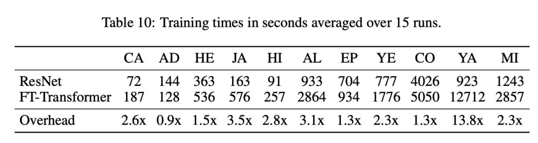
Training Time

Firstly, the authors present a comparison of the training time between ResNet and FT-Transformer on the 11 datasets discussed:

Next, the authors attempted to limit the tuning time and observe the performance of different models. In this experiment, XGBoost, MLP, ResNet, and FT-Transformer were used. The experiment was conducted on three datasets: California Housing, Adult, and Higgs Small. The results are as follows:

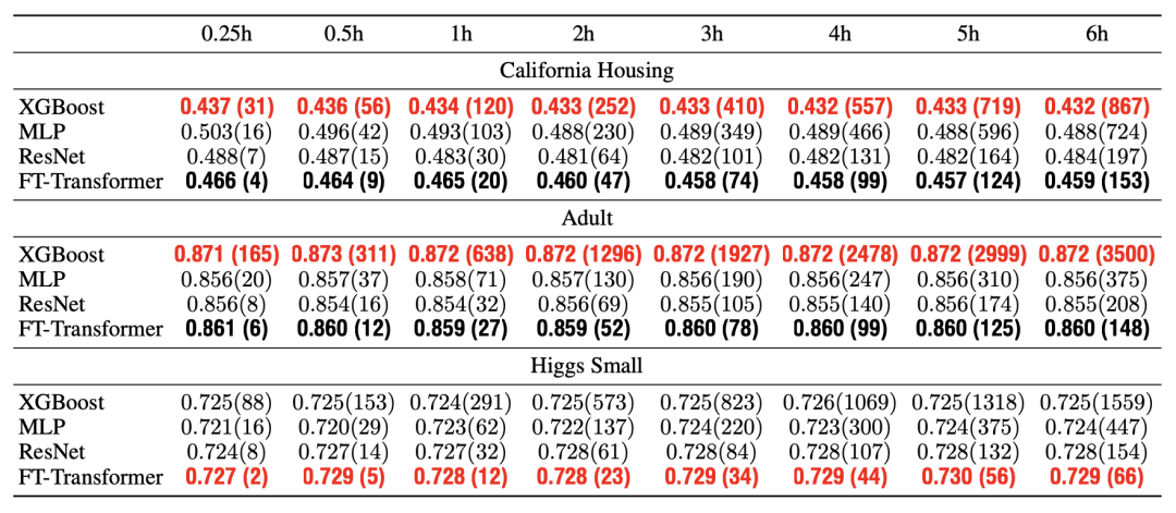
Limit training time comparison — Figure 11. The number of iterations for tuning with Optuna is indicated in parentheses. The red bold font represents the best performance among all models, while the black bold font represents the best performance among the deep learning models.

It can be observed that:

FT-Transformer performs well in a few rounds of random parameter selection (within the first 10 rounds of default random selection with Optuna).
FT-Transformer has a slower training speed compared to other models.
Additional iterations have limited significance for other models.

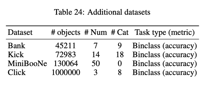
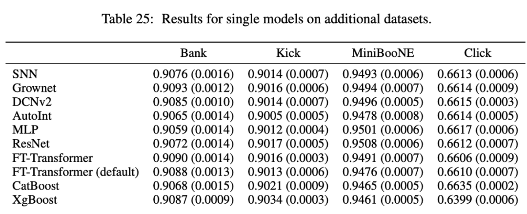
Other datasets

The appendix provides the performance of different models on four datasets that were not mentioned in the main text. The author found that all models perform similarly on these datasets, but the limited information provided does not warrant their inclusion in the main text. The four datasets are as follows:

Review comments

From the openreview, we can see the questions raised by the reviewers before the paper was accepted. Some of the answers to these questions are already reflected in the appendix, such as the changes in model performance over time and the datasets like “click.” However, I would like to highlight the question regarding the selection of GBDT models.

One comment mentioned that both XGBoost and CatBoost use level-wise trees, and it would be interesting to explore the use of leaf-wise trees like LightGBM.

The author provided experiment results on LightGBM:

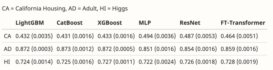
LightGBM for comparison — Figure 13. Comparison of LightGBM and other models on CA, AD, HI datasets.

CA and AD are datasets where GBDT performs well, and HI is a dataset where deep learning and GBDT perform similarly. For CA, lower values are better, while higher values are better for the other two. It can be observed that LightGBM performs similarly to the other two GBDT models, which aligns with the author’s expectations.

The author mentioned that deep learning models were not able to surpass GBDT on datasets that are more favorable to GBDT. Therefore, additional GBDT models were not included. However, if deep learning models start to outperform some GBDT models on datasets that are more GBDT-friendly, it would be necessary to include more GBDT models for comparison.

Implementation

The article provides a comprehensive comparison and answers questions that have long puzzled me. Yandex is a Russian search giant, and CatBoost is also from this company, which is worth paying attention to.

At the same time, I have learned two new things: FT-Transformer and Optuna. I have tried both tools personally, and I would like to share the code for each.

ft_transformer.py:

import math
from unicodedata import name
from gzip import GzipFile
import torch 
import torch.nn as nn 
from sklearn.model_selection import train_test_split
from sklearn.preprocessing import StandardScaler, quantile_transform
from sklearn.metrics import classification_report, accuracy_score 
import numpy as np 
import pandas as pd 
import os 
from tqdm import tqdm
import matplotlib.pyplot as plt 
from collections import deque


class PositionalEncoding(nn.Module):
    def __init__(self, d_model, dropout=0.1, max_len=5000):
        super(PositionalEncoding, self).__init__()
        self.dropout = nn.Dropout(p=dropout)
        pe = torch.zeros(max_len, d_model)
        position = torch.arange(0, max_len, dtype=torch.float).unsqueeze(1)
        div_term = torch.exp(torch.arange(0, d_model, 2).float() * (-np.log(10000.0) / d_model))
        pe[:, 0::2] = torch.sin(position * div_term)
        pe[:, 1::2] = torch.cos(position * div_term)
        pe = pe.unsqueeze(0).transpose(0, 1)
        self.register_buffer('pe', pe)

    def forward(self, x):
        '''
        x: [sequence length, batch size, embed dim]
        output: [sequence length, batch size, embed dim]
        '''
        x = x + self.pe[:x.size(0), :]
        return self.dropout(x)


class CatNumerDataset(torch.utils.data.Dataset):
    def __init__(self, cats_data, numers_data, labels):
        super().__init__()
        self.cats_data = cats_data
        self.numers_data = numers_data
        self.labels = labels 
        self.length = len(cats_data)
    

    def __getitem__(self, index):
        return self.cats_data[index], self.numers_data[index], self.labels[index]


    def __len__(self):
       return self.length         


class NumerFeatureTokenizer(nn.Module):
    def __init__(
        self,
        feature_dim, 
        embedding_dim,
        device
        ):
        super().__init__()
        
        self.feature_dim = feature_dim
        self.embedding_dim = embedding_dim
        self.numer_tokenizers = nn.ModuleList([nn.Linear(1, embedding_dim).to(device) for i in range(feature_dim)])
    

    def forward(self, x_numer):
        '''
        x_numer: [batch size, feature dim]
        output: [batch size, feature dim, embedding dim]
        '''
        batch_size = x_numer.size(0)
        assert self.feature_dim == x_numer.size(1), '特征大小不等'
        x_numer = x_numer.unsqueeze(1)
        device = x_numer.device
        tensor_embed = torch.zeros(batch_size, self.feature_dim, self.embedding_dim, device=device)
        
        for i, idx in enumerate(range(self.feature_dim), start=0):
            tensor_embed[:, i] = self.numer_tokenizers[i](x_numer[:, :, idx])
             
        return tensor_embed


class CatFeatureTokenizer(nn.Module):
    def __init__(
        self,
        max_cats, 
        embedding_dim,
        device
        ):
        super().__init__()
        
        self.feature_dim = len(max_cats)
        self.embedding_dim = embedding_dim
        self.cat_tokenizers = nn.ModuleList([nn.Embedding(max_cats[i], embedding_dim).to(device) for i in range(self.feature_dim)])
    

    def forward(self, x_cat):
        '''
        x_cat: [batch size, feature dim]
        output: [batch size, feature dim, embedding dim]
        '''
        batch_size = x_cat.size(0)
        assert self.feature_dim == x_cat.size(1), '特征大小不等'
        device = x_cat.device
        tensor_embed = torch.zeros(batch_size, self.feature_dim, self.embedding_dim).to(device)
        for i, idx in enumerate(range(self.feature_dim), start=0):
            tensor_embed[:, i] = self.cat_tokenizers[i](x_cat[:, idx])
             
        return tensor_embed


class TransformerClassifier(nn.Module):
    def __init__(
        self, 
        num_classes,
        cat_tokenizer: CatFeatureTokenizer = None,
        numer_tokenizer: NumerFeatureTokenizer = None,
        nhead=8,
        dim_feedforward: int = None,
        dim_feedforward_size_factor: float = 4 / 3,
        dropout=0.1,
        num_layers=3,
        norm=None, 
        batch_first=True
        ):
        super(TransformerClassifier, self).__init__()

        self.cat_tokenizer = cat_tokenizer
        self.numer_tokenizer = numer_tokenizer

        if cat_tokenizer and numer_tokenizer:
            assert cat_tokenizer.embedding_dim == numer_tokenizer.embedding_dim, 'inconsistent tokenizer dimensions'
            d_model = cat_tokenizer.embedding_dim
        elif cat_tokenizer:
            d_model = cat_tokenizer.embedding_dim
        elif numer_tokenizer:
            d_model = numer_tokenizer.embedding_dim
        else:
            raise ValueError('at least one tokenizer is needed')

        
        assert d_model % nhead == 0, 'd_model % nhead != 0'
        self.d_model = d_model
        if dim_feedforward is None:
            dim_feedforward = int(dim_feedforward_size_factor * d_model)
        encoder_layer = nn.TransformerEncoderLayer(batch_first=batch_first, d_model=d_model, nhead=nhead, dim_feedforward=dim_feedforward, dropout=dropout)
        self.transformer_encoder = nn.TransformerEncoder(encoder_layer, num_layers=num_layers, norm=norm)
        self.classifier = nn.Linear(d_model, num_classes)
        self.activation = nn.ReLU()

    def forward(self, x):
        '''
        x: (x_cats, x_numer) tuple; or x_cats/ x_numer tensor
        shape: [batch_size, feature_dim, embedding_dim]
        output: [batch_size, num_classes]
        '''
        if isinstance(x, tuple):
            if self.numer_tokenizer and self.cat_tokenizer:
                x_cats, x_numer = x 
                x_cats = self.cat_tokenizer(x_cats)
                x_numer = self.numer_tokenizer(x_numer)
                x = torch.hstack([x_cats, x_numer])
            else:
                raise ValueError(f'Tokenizer not found')
        else:
            if self.cat_tokenizer:
                x = self.cat_tokenizer(x)
            if self.numer_tokenizer:
                x = self.numer_tokenizer(x)

        batch_size = x.shape[0]  
        device = x.device      
        cls = torch.zeros(batch_size, 1, self.d_model, device=device)
        x = torch.hstack([cls, x])
        # self.temp = x 
        x = self.transformer_encoder(x)
        # self.tmp = x 
        # x = x.mean(dim=1)
        cls = x[:, 0, :]
        cls = self.activation(cls)
        y_pred = self.classifier(cls)
        return y_pred


def train(model: TransformerClassifier, train_loader, val_loader, criterion, optimizer, device, num_epochs: int = 3, save_to: str = os.path.join('model', 'transformer_val_best_model'), is_lstm = False):
    loss_trace = []
    best_val_loss = np.inf
    best_val_score = 0
    for epoch in tqdm(range(num_epochs)):
        model.train()
        current_loss = 0
        for i, (x_cat_batch, x_numer_batch, y_batch) in enumerate(train_loader):
            x_cat_batch, x_numer_batch, y_batch  = x_cat_batch.to(device), x_numer_batch.to(device), y_batch.to(device)
            if is_lstm:
                x = torch.cat([x_cat_batch, x_numer_batch], dim=2).to(dtype=torch.float32)
                pred = model(x)
            else:
                pred = model((x_cat_batch, x_numer_batch.to(dtype=torch.float32)))
            loss = criterion(pred, y_batch.to(dtype=torch.int64))
            optimizer.zero_grad()
            loss.backward()
            optimizer.step()
            current_loss += loss.item()
        loss_trace.append(current_loss)

        model.eval()
        val_loss = 0
        val_score = deque()
        pred_val = deque()
        with torch.no_grad():
            for x_cat_batch, x_numer_batch, y_batch in val_loader:
            
                x_cat_batch, x_numer_batch, y_batch  = x_cat_batch.to(device), x_numer_batch.to(device), y_batch.to(device)
                if is_lstm:
                    x = torch.cat([x_cat_batch, x_numer_batch], dim=2).to(dtype=torch.float32)
                    pred = model(x)
                else:
                    pred = model((x_cat_batch, x_numer_batch.to(dtype=torch.float32)))
                pred_batch = torch.argmax(pred, dim=1).cpu().numpy()
                pred_val.append(pred_batch)
                val_score.append(y_batch.cpu().numpy())
                loss = criterion(pred, y_batch.to(dtype=torch.int64))
                val_loss += loss.item()
            # val_loss = np.mean(val_loss)
        
        val_score = accuracy_score(np.hstack(val_score), np.hstack(pred_val))
        
        print(f'epoch: {epoch} \n val loss: {val_loss} \t train loss: {current_loss} \n val score: {val_score}')

        if val_loss < best_val_loss or val_score > best_val_score:
            torch.save(
            {
                'epoch': epoch,
                'model_state_dict': model.state_dict(),
                'best_val_loss': val_loss,
                'best_val_score': val_score
            }, 
            save_to
            )
            print('model saved')
            if val_loss < best_val_loss:
                best_val_loss = val_loss
            if val_score > best_val_score:
                best_val_score = val_score

        torch.save(
            {
                'epoch': 'last',
                'model_state_dict': model.state_dict()
            }, 
            os.path.join('model', 'transformer_last_epoch')
            )
    # loss curve
    plt.plot(range(1, num_epochs+1), loss_trace, 'r-')
    plt.xlabel('Epoch')
    plt.ylabel('Loss')
    plt.show()  
        

def evaluate(model, test_loader, device, is_lstm=False):
    # to_load = os.path.join('model', 'transformer_val_best_model')
    # model.load_state_dict(torch.load(to_load)['model_state_dict'])
    model.eval()
    pred_result, true_result = deque(), deque()

    with torch.no_grad():
        for x_cat_batch, x_numer_batch, y_batch in tqdm(test_loader):    
            x_cat_batch, x_numer_batch, y_batch  = x_cat_batch.to(device), x_numer_batch.to(device), y_batch.to(device)
            if is_lstm:
                x = torch.cat([x_cat_batch, x_numer_batch], dim=2).to(dtype=torch.float32)
                pred = model(x)
            else:
                pred = model((x_cat_batch, x_numer_batch.to(dtype=torch.float32)))
            pred_batch = torch.argmax(pred, dim=1).cpu().numpy()
            pred_result.append(pred_batch)
            true_result.append(y_batch.cpu().numpy())

    true_result = np.hstack(true_result)
    pred_result = np.hstack(pred_result)
    print(classification_report(true_result, pred_result)) 
    score = accuracy_score(true_result, pred_result)
    return score
    

if __name__ == '__main__':
    device = torch.device("cuda:0" if torch.cuda.is_available() else "cpu")
    os.makedirs('model', exist_ok=True)
    np.random.seed(44)
    try:
        Xy = np.genfromtxt(GzipFile(filename='covtype.data.gz'), delimiter=",")
        X = Xy[:, :-1]
        y = Xy[:, -1].astype(np.int32, copy=False)
        y -= 1

        x_numers = X[:, :10]

        x_cats = X[:, 10:]
        x_cat1 = x_cats[:, :4].argmax(axis=1).copy()
        x_cat2 = x_cats[:, 4:].argmax(axis=1).copy()
        x_cat = np.vstack([x_cat1, x_cat2]).T.copy()
        test_ratio = 0.2
        val_ratio = 0.2
        x_n_train, x_n_test, x_c_train, x_c_test, y_train, y_test = train_test_split(x_numers, x_cat, y, test_size=test_ratio, stratify=y, random_state=44)
        x_n_train, x_n_val, x_c_train, x_c_val, y_train, y_val = train_test_split(x_n_train, x_c_train, y_train, test_size=val_ratio, stratify=y_train, random_state=44)

        preprocess_n = StandardScaler().fit(x_n_train)
        x_n_train, x_n_val, x_n_test = torch.tensor(preprocess_n.fit_transform(x_n_train), device=device), torch.tensor(preprocess_n.fit_transform(x_n_val), device=device), torch.tensor(preprocess_n.fit_transform(x_n_test), device=device)
        train_dataset = CatNumerDataset(x_c_train, x_n_train, y_train)
        val_dataset = CatNumerDataset(x_c_val, x_n_val, y_val)
        test_dataset = CatNumerDataset(x_c_test, x_n_test, y_test)

        batch_size = 256
        train_loader = torch.utils.data.DataLoader(train_dataset, batch_size = batch_size)
        val_loader=  torch.utils.data.DataLoader(val_dataset, batch_size=batch_size)
        test_loader = torch.utils.data.DataLoader(test_dataset, batch_size = batch_size)

        embedding_dim = 192
        cft = CatFeatureTokenizer(max_cats=[4, 40], embedding_dim=embedding_dim, device=device)
        nft = NumerFeatureTokenizer(feature_dim=10, embedding_dim=embedding_dim, device=device)
        model = TransformerClassifier(num_classes=7, dropout=0.2, cat_tokenizer=cft, numer_tokenizer=nft).to(device)

        lr = 0.0001
        criterion = nn.CrossEntropyLoss()
        optimizer = torch.optim.AdamW(model.parameters(), lr = lr)

        train(model, train_loader, val_loader, criterion, optimizer, device)
        evaluate(model, test_loader, device)
    except FileNotFoundError:
        print('Data not found.')

As for optuna.ipynb:

import math
import optuna
import torch  # torch.__version__ >= 1.9.0
import torch.nn as nn 
from sklearn.model_selection import train_test_split
from sklearn.preprocessing import StandardScaler
from sklearn.metrics import classification_report, accuracy_score 
from gzip import GzipFile
import numpy as np 
import os 
from tqdm import tqdm
import matplotlib.pyplot as plt 
from collections import deque

from ft_transformer import NumerFeatureTokenizer, CatFeatureTokenizer, TransformerClassifier

device = torch.device("cuda:0" if torch.cuda.is_available() else "cpu")
os.makedirs('model', exist_ok=True)
np.random.seed(44)

Read and pre-process the data

Xy = np.genfromtxt(GzipFile(filename='covtype.data.gz'), delimiter=",")

X = Xy[:, :-1]
y = Xy[:, -1].astype(np.int32, copy=False)
y -= 1

x_numers = X[:, :10]
x_cats = X[:, 10:]
x_cat1 = x_cats[:, :4].argmax(axis=1).copy()
x_cat2 = x_cats[:, 4:].argmax(axis=1).copy()
x_cats = np.vstack([x_cat1, x_cat2]).T.copy()

test_ratio = 0.2
val_ratio = 0.2
x_n_train, x_n_test, x_c_train, x_c_test, y_train, y_test = train_test_split(x_numers, x_cats, y, test_size=test_ratio, stratify=y, random_state=44)
x_n_train, x_n_val, x_c_train, x_c_val, y_train, y_val = train_test_split(x_n_train, x_c_train, y_train, test_size=val_ratio, stratify=y_train, random_state=44)

preprocess_n = StandardScaler().fit(x_n_train)
x_n_train, x_n_val, x_n_test = torch.tensor(preprocess_n.fit_transform(x_n_train), device=device), torch.tensor(preprocess_n.fit_transform(x_n_val), device=device), torch.tensor(preprocess_n.fit_transform(x_n_test), device=device)

Dataloader:

class CatNumerDataset(torch.utils.data.Dataset):
    def __init__(self, cats_data, numers_data, labels) -> None:
        super().__init__()
        self.cats_data = cats_data
        self.numers_data = numers_data
        self.labels = labels 
        self.length = len(cats_data)
    

    def __getitem__(self, index):
        return self.cats_data[index], self.numers_data[index], self.labels[index]


    def __len__(self):
        return self.length   

train_dataset = CatNumerDataset(x_c_train, x_n_train, y_train)
val_dataset = CatNumerDataset(x_c_val, x_n_val, y_val)
test_dataset = CatNumerDataset(x_c_test, x_n_test, y_test)

batch_size = 256
train_loader = torch.utils.data.DataLoader(train_dataset, batch_size = batch_size)
val_loader=  torch.utils.data.DataLoader(val_dataset, batch_size=batch_size)
test_loader = torch.utils.data.DataLoader(test_dataset, batch_size = batch_size)

#  subset of dataset for tutorial
subset_train_indices = torch.randperm(len(train_dataset))[:3000]
subset_val_indices = torch.randperm(len(val_dataset))[:3000]
train_sampler = torch.utils.data.SubsetRandomSampler(subset_train_indices)
val_sampler = torch.utils.data.SubsetRandomSampler(subset_val_indices)
subset_train_loader = torch.utils.data.DataLoader(train_dataset, batch_size=batch_size, sampler=train_sampler)
subset_val_loader = torch.utils.data.DataLoader(val_dataset, batch_size=batch_size, sampler=val_sampler)

Supportive functions for optuna:

classes = 7
in_features = 10
max_cats = [4, 40]

def build_fttransformer(trial, num_classes: int, feature_dim: int, max_cats: list, embedding_dim: int = 192, device=device, **kwargs):
    embedding_dim = trial.suggest_int('embedding_dim', 160, 512, 16)
    dropout = trial.suggest_float('dropout', 0.2, 0.5)
    
    cft = CatFeatureTokenizer(max_cats=max_cats, embedding_dim=embedding_dim, device=device)
    nft = NumerFeatureTokenizer(feature_dim=feature_dim, embedding_dim=embedding_dim, device=device)
    model = TransformerClassifier(num_classes=num_classes, cat_tokenizer=cft, numer_tokenizer=nft, dropout=dropout, **kwargs)
    return model

#  MLP model
class MLPClassifier(nn.Module):
    def __init__(self, num_classes: int, n_layers: int = 3,
                 hidden_size: int = 64,
                 cat_tokenizer: CatFeatureTokenizer = None,
                 numer_tokenizer: NumerFeatureTokenizer = None):
        super(MLPClassifier, self).__init__()

        self.cat_tokenizer = cat_tokenizer
        self.numer_tokenizer = numer_tokenizer
        
        if cat_tokenizer and numer_tokenizer:
            assert cat_tokenizer.embedding_dim == numer_tokenizer.embedding_dim, 'Inconsistent tokenizer dimensions'
            d_model = cat_tokenizer.embedding_dim
        elif cat_tokenizer:
            d_model = cat_tokenizer.embedding_dim
        elif numer_tokenizer:
            d_model = numer_tokenizer.embedding_dim
        else:
            ValueError('At least one tokenizer is required')
        
        self.input_size = d_model
        self.hidden_size = hidden_size
        self.num_classes = num_classes
        
        self.activation = nn.ReLU()
        self.classifier = nn.Linear(self.hidden_size, self.num_classes)
        
        self.layers = nn.ModuleList()
        for i in range(n_layers):
            if i == 0:
                self.layers.append(nn.Linear(self.input_size, self.hidden_size))
            else:
                self.layers.append(nn.Linear(self.hidden_size, self.hidden_size))
            self.layers.append(self.activation)
            
        
    def forward(self, x):
        '''
        x: (x_cats, x_numer) tuple; or x_cats/ x_numer tensor
        shape: [batch_size, feature_dim, embedding_dim]
        output: [batch_size, num_classes]
        '''
        if isinstance(x, tuple):
            if self.numer_tokenizer and self.cat_tokenizer:
                x_cats, x_numer = x 
                x_cats = self.cat_tokenizer(x_cats)
                x_numer = self.numer_tokenizer(x_numer)
                x = torch.hstack([x_cats, x_numer])  # hstack available in version 1.8.0
#                 x = torch.cat([x_cats, x_numer], dim=1)
            else:
                ValueError(f'Tokenizer not found')
        else:
            if self.cat_tokenizer:
                x = self.cat_tokenizer(x)
            if self.numer_tokenizer:
                x = self.numer_tokenizer(x)

        batch_size = x.shape[0]  
        device = x.device      
        
        for module in self.layers:
            x = module(x)
        x = x.mean(dim=1)
        y_pred = self.classifier(x)
        return y_pred 

def build_mlp(trial, num_classes: int, feature_dim: int, embedding_dim: int = 192, device = device):
    
    cft = CatFeatureTokenizer(max_cats=max_cats, embedding_dim=embedding_dim, device=device)
    nft = NumerFeatureTokenizer(feature_dim=feature_dim, embedding_dim=embedding_dim, device=device)
    # We optimize the number of layers.
    n_layers = trial.suggest_int("n_layers", 1, 3)
    model = MLPClassifier(num_classes=num_classes, n_layers=n_layers, cat_tokenizer=cft, numer_tokenizer=nft)
    return model

def build_model(trial):
    model_name = trial.suggest_categorical('model_name', ['mlp', 'fttransformer'])
    if model_name == 'mlp':
        return build_mlp(trial, classes, in_features)
    if model_name == 'fttransformer':
        return build_fttransformer(trial, classes, in_features, max_cats)

def train_evaluate(trial, model, train_loader, val_loader, criterion, optimizer, num_epochs: int = 3):
    for epoch in tqdm(range(num_epochs)):
        model.train()
        current_loss = 0
        for i, (x_cat_batch, x_numer_batch, y_batch) in enumerate(train_loader):
            x_cat_batch, x_numer_batch, y_batch  = x_cat_batch.to(device), x_numer_batch.to(device), y_batch.to(device)
            pred = model((x_cat_batch, x_numer_batch.to(dtype=torch.float32)))
            loss = criterion(pred, y_batch.to(dtype=torch.int64))
            optimizer.zero_grad()
            loss.backward()
            optimizer.step()
            current_loss += loss.item()

        model.eval()
        val_score = deque()
        pred_val = deque()
        with torch.no_grad():
            for x_cat_batch, x_numer_batch, y_batch in val_loader:
            
                x_cat_batch, x_numer_batch, y_batch  = x_cat_batch.to(device), x_numer_batch.to(device), y_batch.to(device)
                pred = model((x_cat_batch, x_numer_batch.to(dtype=torch.float32)))
                pred_batch = torch.argmax(pred, dim=1).cpu().numpy()
                pred_val.append(pred_batch)
                val_score.append(y_batch.cpu().numpy())
                loss = criterion(pred, y_batch.to(dtype=torch.int64))
        
        val_score = accuracy_score(np.hstack(val_score), np.hstack(pred_val))

        trial.report(val_score, epoch)
        if trial.should_prune():
            raise optuna.exceptions.TrialPruned()
            
    return val_score 

def objective(trial):
    
    params = {
        'lr': trial.suggest_loguniform('lr', 1e-5, 1e-1),
        'optimizer_name': trial.suggest_categorical('optimizer', ['AdamW', 'Adam', 'SGD']),
    }
    model = build_model(trial).to(device)
    
    optimizer = getattr(torch.optim, params['optimizer_name'])(model.parameters(), lr=params['lr'])
    criterion = nn.CrossEntropyLoss()
    score = train_evaluate(trial, model, subset_train_loader, subset_val_loader, criterion, optimizer)

    return score 

Run experiments:

study = optuna.create_study(direction='maximize')
study.optimize(objective, n_trials=50, timeout=600)

pruned_trials = study.get_trials(deepcopy=False, states=[optuna.trial.TrialState.PRUNED])
complete_trials = study.get_trials(deepcopy=False, states=[optuna.trial.TrialState.COMPLETE])

print("Study statistics: ")
print("  Number of finished trials: ", len(study.trials))
print("  Number of pruned trials: ", len(pruned_trials))
print("  Number of complete trials: ", len(complete_trials))

print("Best trial:")
trial = study.best_trial

print("  Value: ", trial.value)

print("  Params: ")
for key, value in trial.params.items():
    print("    {}: {}".format(key, value))

Check my post on Discovery Lab: 【每周一读】重提表格数据上的深度学习

Share on

Twitter Facebook LinkedIn

Bowen Fang