Can deep reinforcement learning algorithms be used to train a trading agent that can achieve long-term profitability using Limit Order Book (LOB) data? To answer this question, this article proposes a deep reinforcement learning framework for high-frequency trading and conducts experiments using limit order data from LOBSTER with the PPO algorithm. The results show that the agent is able to identify short-term patterns in the data and propose profitable trading strategies.

Original Paper Information
Title: Deep Reinforcement Learning for Active High Frequency Trading
Author: Antonio Briola, Jeremy Turiel, Riccardo Marcaccioli, Tomaso Aste
DOI: arXiv:2101.07107

Background

Limit Order Book

A Limit Order Book (LOB) records the outstanding limit orders in the current market. A limit order is an order with a specified price that is not lower than the specified price. The LOB data used in the article refers to the ten-level market data, which includes the top ten buy and sell prices with the highest priority, as well as the total order quantity at each price level. The difference between the best bid price and the best ask price is referred to as the bid-ask spread.

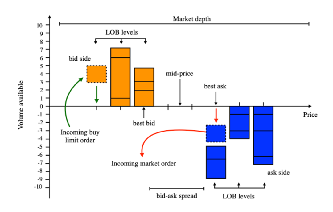
Traders buy or sell securities by sending instructions to the exchange in the form of limit orders or market orders. These instructions are stored in two separate queues based on the buy or sell direction until they are either canceled or executed. Each order, denoted as $x$, contains four pieces of information: buy/sell direction ($\epsilon_x$), limit price ($p_x$), order quantity ($V_x$), and order arrival time ($τ_x$). Currently, most exchanges employ a price-time priority rule, where higher bid orders have priority over lower bid orders, and lower ask orders have priority over higher ask orders. For orders with the same price, the order that arrives first is given priority. Market orders, on the other hand, bypass the bid-ask spread and are typically executed immediately, at the cost of bearing the crossing spread as a trading cost. Therefore, the bid-ask spread is referred to as the trading cost for market orders.

PPO

The PPO algorithm is a type of Policy Gradient algorithm and falls under the category of on-policy methods. Compared to previous algorithms such as REINFORCE, PPO improves by controlling the update step size of the policy to prevent it from being too large, which could cause the model to collapse, or too small, which could result in excessively long training times. PPO inherits the idea of controlling policy updates from TRPO but offers easier implementation and lower computational complexity, surpassing TRPO in performance. PPO also has different implementation variants, with the clip-based approach being more common. The objective function for PPO with the clip-based approach is as follows: \(\newcommand{\clip}{\mathrm{clip}}\) \(\begin{align} L(\theta) & = \mathbb{E}_t[\min(r_t(\theta)A_t, \clip(r_t(\theta),1-\epsilon,1+\epsilon)A_t)] \\ r_t(\theta) & = \frac{\pi_\theta(a_t|s_t)}{\pi_{\theta_{old}}(a_t|s_t)} \end{align}\)

Where $A_t$ represents the advantage function, which is a function of the action and state. It is defined as the difference between the Q-value of action $a$ and the value of state $s$ under the policy $\pi$. It reflects the performance of action $a$ compared to the average. $\pi$ represents the policy, and $θ$ represents the parameters of the policy network, which outputs the probability of selecting action $a$ given state $s$. $r_t$ represents the ratio of the probabilities of the new policy and the old policy. The clip function ensures that $r_t$ does not exceed the range $[1-ε, 1+ε]$.

The interpretation is as follows: when $A > 0$, it indicates that action a has an advantage over other actions, so the policy network should increase the output probability of action $a$, which means increasing $r_t$. However, $r_t$ should not exceed $1+ε$. When $A < 0$, it indicates that action $a$ is at a disadvantage compared to other actions, so the network should decrease the output probability, but not below $1-ε$.

Method

Data

The data used in this paper comes from LOBSTER, which provides tick-by-tick and snapshot data for all stocks on the NASDAQ exchange. The snapshot data of INTC was used for the subsequent experiments because, relatively speaking, trading in large stocks is more active and price changes are more dependent on the information in LOB. The duration of the data used is 60 trading days, with the training set covering the period from 2019/02/04 to 2019/04/30, the validation set covering 2019/05/01 to 2019/05/31, and the test set covering 2019/06/03 to 2019/06/28. Due to the instability during the opening and closing periods, the data for the initial and last 2*10^5 ticks of each trading day were excluded.

Model

3 different state definitions are tested, which are:

• $s_{201}$: current and most recent 9 ticks 10-level buy-sell volume and current long/short state;
• $s_{202}$: $s_{201}+$ current profit earned if closing position (current price - opening price, spread considered);
• $s_{203}$: $s_{202}+$ current spread

4 actions (\(\mathcal{A}=\{0:sell, 1:stay, 2:long, 3:daily\ stop\ loss\}\)) for the agent, which based on the state of the position(\(\mathcal{P}=\{N:neutral,L:long,S:short\}\)), result in different effect:

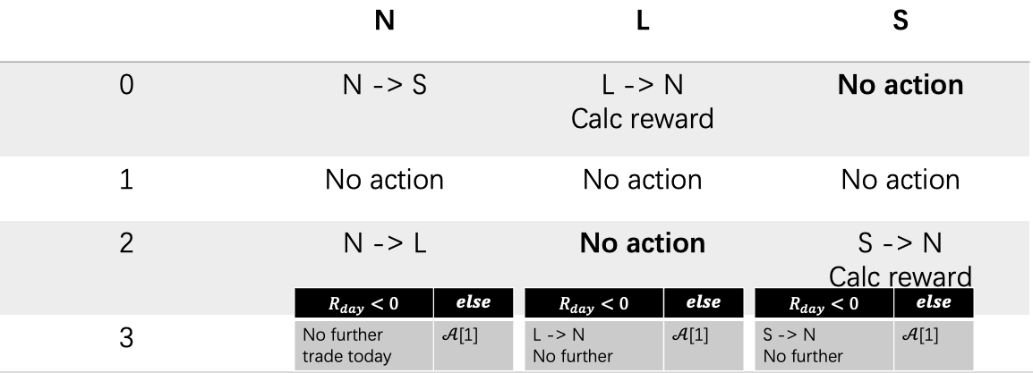
Regardless of whether there is a position or not, Action 1 does nothing. If there is no current position, Actions 0 and 2 respectively initiate a sell and buy of the minimum trading unit, entering a short and long position. Regardless of whether there is a position or not, Action 3 calculates the cumulative profit at the current moment. If it is less than 0, the position is closed; otherwise, no action is taken. If the current position is short, Action 0 does nothing, and Action 2 buys the minimum trading unit to close the short position and calculates the trading profit. If the current position is long, Action 2 does nothing, and Action 0 sells to close the long position and calculates the trading profit.

The calculation of trading profit, as defined in this paper, is based on the position entered at time ($\tau - t$) and closed at time $\tau$, and the profit is calculated as follows:

Where $l/s$ represents long and short, \(p^{best}_{a,\tau},p^{best}_{b,\tau}\) represents the best ask and bid price at time $\tau$.

Note that the model proposed trades and holds only one unit of stock asset at each time point. This assumption is made for several reasons: trading itself can impact the Limit Order Book (LOB), larger trades may cause significant changes in the mid-price; larger trading orders are typically split into multiple smaller orders for execution; and introducing a variable for the number of units traded would require a more complex model.

Pipeline

In the training phase, for each trading day, a window of $10^4$ consecutive ticks is selected, and 5 segments with the largest absolute mid-price changes are chosen. From all the segments, 25 are selected to form the vectorized DRL environment. Each environment undergoes 30 epochs of iteration.

The reason for this approach is that the paper believes larger price changes offer more opportunities for trading actions.

The agent policy and value network share parameters and are implemented as a 2-hidden-layer MLP, with separate outputs for action $a$ and value $V$.

In the validation phase, Bayesian optimization is used to tune the model hyperparameters, based on the cumulative returns on the validation set, to determine the next set of parameters. The validation set is processed in the same way as the training set.

In the testing phase, the strategy is independently tested on each day, and trading returns are recorded for plotting the Profit and Loss (P&L) curve.

Result

The following figures depict the performance of the agent on the test set. They include the cumulative P&L curve over the entire test set, the daily average P&L and standard deviation across different iteration rounds, and the distribution of returns for each trade conducted by the agent.

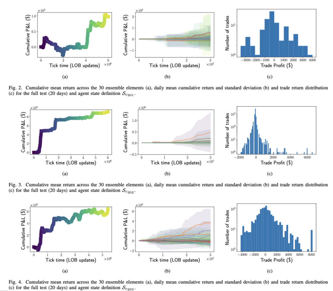
From top to bottom, they correspond to the three different states proposed in the model: 201/202/203. On average, the agent can achieve profitable trading strategies without considering trading costs. Comparing the three different states, the information introduced in state 202 significantly improves trading performance compared to state 201. However, state 203 does not show further improvement over state 202.

From the second column, it can be observed that there are more positive return trading days than negative return trading days, and the realized returns are not concentrated on specific trading days. They are also not affected by intraday cyclic factors.

From the third column, it can be seen that due to the intraday stop-loss action (action 3), the tails of negative returns are truncated. The number of trades in state 202 is significantly higher than in states 201/203.

Comment

This paper demonstrates an approach to applying deep reinforcement learning models to high-frequency trading. It compares and explores the impact of different state designs on out-of-sample performance and discovers that introducing mark-to-market (realizing profits upon closing a position) can enhance the performance of the agent.

The article may have an error in the definition of trading profits. I believes that the correct definition should be \(R_{i,\tau}=\begin{cases} p^{best}_{b,\tau}-p^{best}_{\alpha,\tau-t} & \text{if } i=l \\ p^{best}_{b,\tau-t}-p^{best}_{\alpha, \tau} & \text{if } i=s \end{cases}\)

In order to achieve immediate execution at the prevailing bid/ask spread, the definition of trading profits should be adjusted accordingly.

The paper does not discuss trading delays. Given the trading hours of NASDAQ from 9:30 am to 4:00 pm and the volume of 300,000 ticks of data (as indicated by the x-axis in the second column of the results), it is important to consider the issue of latency when actions are executed.

Furthermore, the article only utilizes “volume” data for the first 200 dimensions of the state design. It may be interesting to explore the impact of incorporating some “price” information, such as the average opening price over the past 5 days, on the performance of the model.

My question pertains to the observed imbalance in action distribution, where a large number of actions result in either no change (1) or the same direction (0 or 2). While the preprocessing method employed in the article’s training set partially addresses this issue, I wonder if there are other approaches to mitigate this problem.

Check my post on Discovery Lab: 【每周一读】深度强化学习在高频交易上的应用